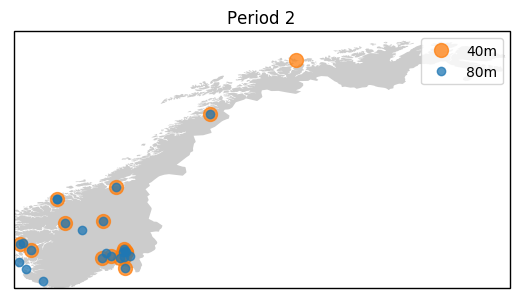
In the post about the Norwegian telephony contest, we plotted the contacts on a map of Norway. Plotting contacts during short time periods like this can give a good visualization on the propagation conditions. In this particular case, it could yield some pointers on how we might do better the next time we run a similar contest. Due to sparse settlement patterns in Norway, however, this mostly demonstrates that Norway is a rather empty country. Regardless, they are nice illustrations :-).
Here, we outline how we did this using Pandas in Python. The more specific details apply only to Norwegian ham radio contacts, as we have used Norway’s database over the address information for Norwegian licensees. It could be applicable to other countries as well, given similar databases and some small tweaking to the scripts.
We will go through it step by step. First, we import all necessary libraries. Pandas for convenient data wrangling:
import pandas as pd
The Nomantim submodule of Geopy for conversion of addresses to coordinates using OpenStreetMap:
from geopy.geocoders import Nominatim
Matplotlib and cartopy for plotting of the data points on a nice map:
import matplotlib.pyplot as plt
import cartopy.crs as ccrs
import cartopy.io.shapereader as shpreader
We could also have used Basemap, but in my short experience, cartopy seems to produce maps that have a lower threshold for looking nice by accident, with a bit more convenient API. This is probably extremely subjective :-).
First, we use the N1MM database reader introduced in a previous post to read the logs into a Pandas dataframe. Since we don’t need all the fields, we remove everything except for the callsign, timestamp and band fields.
qsos = analyze_logs.get_n1mm_logs_in_path('path_to_logs/')[['Call', 'TS', 'Band']]
We then download the official Norwegian ham database, which exists as an Excel sheet and a CSV file. This can conveniently be read using Pandas.read_excel(...), but in order to automatize the joining of this information and the QSO log, we’ll also rename the Norwegian ‘Kallesignal’-column to have the same name as the corresponding column in the QSO log, ‘Call’.
lahamsin = pd.read_excel('Liste over norske radioamatører (Excel) 03.10.2017.xlsx').rename(columns={'Kallesignal': 'Call'})
From geopy, we can get a fine granularity of the coordinates down to address level, but we’ll limit ourselves to the postal code in order to heighten the probability of obtaining an actual coordinate match. The address field can have some weird stuff like a post box number. We add the postal code information to the QSO table by running
qsos = pd.merge(qsos, lahamsin[['Call', 'Postnr']], on='Call')
Each contact in the log will now have its corresponding postal code. For conversion to coordinates, we’ll be using geopy.Nominatim(...), which can look up coordinates from addresses using OpenStreetmap. Geopy also has support for various other map APIs, but these typically require API keys or user authentication. We bias the look-up to Norway in order to probably play a bit more nice with the server.
geocoder = Nominatim(format_string='%s, Norway', country_bias='Norway')
Next, we obtain all unique postal numbers from the QSO table in order to limit the number of look-ups we have to do.
addresses = qsos[['Postnr']].drop_duplicates()
We then look up each postal number against the OpenStreetmap API using Pandas.DataFrame.apply(), which can apply a function row by row to the dataframe. In this case,
geocoder.geocode(...) is used to look up coordinates from the postal code in each row, assuming Norway as the country.
addresses["geocoder_res"] = addresses.apply(lambda x: geocoder.geocode({'postalcode': x.Postnr, 'country': 'Norway'}), axis=1)
Latitudes and longitudes are extracted in a similar way.
addresses['longitude'] = addresses.apply(lambda x: x.geocoder_res.longitude if x.geocoder_res is not None else None, axis=1)
addresses['latitude'] = addresses.apply(lambda x: x.geocoder_res.latitude if x.geocoder_res is not None else None, axis=1)
Merging back the addresses by joining on the postal code, we finally get a complete QSO table including the longitude/latitude coordinates of each contact.
qsos = pd.merge(qsos, addresses.drop('geocoder_res', axis=1), on='Postnr')
qsos = addresses.drop(['Postnr'], axis=1)
Now that we have wrangled all the data, we can finally turn to plotting :-). It can probably be a good idea to save the data to a file in order to avoid having to look up the coordinates against OpenStreetMap every time the script is run.
Cartopy has in-built support for automatically downloading Natural Earth shapefiles when a specific shapefile is requested (and then avoid having to download it again by caching the file). The shapefiles contains various information like country borders, roads, railroads, …, and can be used to plot the borders of a specific country like e.g. Norway down to various resolutions.
We use the admin_0_countries shapefile from the cultural database at 10 meters resolution.
shapefilename = shpreader.natural_earth(resolution='10m',
category='cultural', name='admin_0_countries')
I have not yet found a nice way to find the geometry shape corresponding to Norway except for looping through all records and stopping at “Norway”. There are probably better ways than this :-).
reader = shpreader.Reader(shapefilename)
countries = list(reader.records())
for country in countries:
   if country.attributes['NAME_LONG'] == 'Norway':
      norway = country.geometry
      break
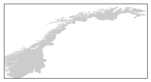
Now that we have the country borders of Norway, we can finally set the borders of Norway and prepare a country map.
projection = ccrs.Mercator()
ax = plt.axes(projection=projection)
ax.add_geometries([norway], projection, facecolor=(0.8, 0.8, 0.8))

Plotting all contacts made on the 80 meters band can then be done using e.g.
band_80m = qsos[qsos.Band == 3.5]
ax.plot(band_80m.longitude.dropna().as_matrix(), band_80m.latitude.dropna().as_matrix(), 'o')
plt.show()
This image is from one of the periods during the Norwegian ham radio contest “Telefonitesten”, and contains the 40m contacts and 80m contacts with different marker colors and sizes.
This should serve as a nice example on how data from three different sources can be combined using Pandas.


Leave a Reply